Great Lakes Bathymetry
From TSAS Library
Revision as of 12:07, 20 August 2017 by JStallings (talk | contribs)
Ideas
- Process of creating a 3D map of the area
- Try this map with these instructions
- For OSM information, use Geofabrik.de and reformat if necessary as described here[1]
Resources
- Downloadable Great Lakes bathymetric maps from NOAA
- All bathymetric maps from NOAA
- The USGS Earth Explorer is easier to use than the above, but requires a login and download client
- Natural Earth provides shapefiles for cultural and physical elements
- Index of one arc-second images from NASA's Shuttle Radar Topography mission
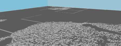
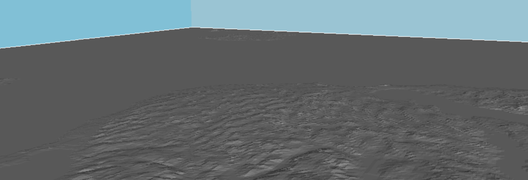
Create STL for CNC Router or 3D Printer
Proprietary Workflow (Aspire)
Video walkthrough here
- Data pulled from NOAA's ETOPO1 images, available directly here which offers a 1-minute resolution of worldwide bedrock
- Add raster image to QGIS
- Select extent desired (Raster -> Extraction -> Clipper)
- Export as .tiff
- Open in GIMP, click white area surrounding with Magic Wand Tool, then drag upward to increase threshold to maximum
- Overwrite .tiff to save
- Open in Aspire, under Modeling tab, select "Create a component from selected bitmap"
- Right-click component under Component Tree, then select Properties
- Switch to 3D view so the changes are illustrated
- Move Shape Height slider until desired relief is achieved (1.5" was used for this project)
- Open unadjusted .tiff in Inkscape (one with dark image with little detail, but sharp boundary edge)
- Choose Path -> Trace Bitmap
- Use Brightness Cutoff with the lowest possible settings
- Deselect Smooth
- Choose Path -> Outset to increase size so bitmap is tightly enveloped by vector (may need to adjust outset steps under Preferences -> Steps)
- Erase any holes within the vector to create solid object
- Import vector in Aspire and carefully align to .tiff
- Move to Toolpaths bar and select 3D Roughing Path
- Choose Selected Vector under Machining Limit Boundary, then press Calculate
- Press 3D Finishing Toolpath, then choose vector as above
- Preview the toolpaths to ensure desired results
- If image is larger than machine, use Tile Toolpaths to divide it [2]
Tool speeds used in above (wooden) image:
| Print Pass | Tool Size | Feed Rate | Plunge Rate | Print Time |
|---|---|---|---|---|
| Rough Pass | .25" square bit | 15.0 mm/sec | 3.0 mm/sec | 1:30 |
| Finish Pass | .125" ball nose | 25.0 mm/sec | 6.0 mm/sec | 4:30 |
Open Source Workflow
- Download ArcGrid DEM from USGS National Map or Earth Explorer (3DEP, 1/3 arc-second DEM)
- Unzip file
- Open QGIS, add Vector, add layer file (.adf)
- Select extent (Raster -> Extraction -> Clipper)
- Save as GeoTIFF
- Add GeoTIFF to model
- Analyze to DEM (Raster -> Analysis -> DEM [Terrain Models])
- If necessary, merge the DEMs
- A balance must be made between extent and resolution. 1:50,000 creates excellent models, but cannot contain an entire lake. Above that and the file crashes my system. A further note on resolution.
- Solution to bathymetric (negative) altitude values[3]: using Raster Calculator, add bottom value to all height values
- Create STL (Raster -> DEMto3D)[4]
Very Long, Detailed Workflow
- Download QGIS
- Download Great Lakes Bathymetry from NOAA's Grid Extract Tool
- Download lakes shapefiles from Science Base
- Open shapefiles in QGIS and merge each at border
- Open first file, e.g. hydro_p_LakeErie.shp
- Right click in Layers Panel and save as LakeEriebound
- Remove original shapefile
- Repeat for all needed
- Select LakeEriebound in Layers Panel, click Select Features by area or single click
- Hold shift, select both features in LakeEriebound on map
- Click Toggle Editing (pencil icon)
- Go to Edit -> Merge Selected Features
- Check that LakeEriebound is now one polygon, Toggle Editing, save changes, then repeat for all shapefiles
- Go to Vector -> Geoprocessing Tools -> Fixed distance buffer
- Run as batch process by inputting each shapefile (LakeEriebound, etc.) into Input Layer, and buffer name (e.g. eriemask) in Buffer column. Used .2 Distance
- Remove LakeEriebound, etc. from Layers Panel
- Add bathymetry rasters from NOAA's Grid Extract Tool, ensuring all area under buffers is included
- Rename Buffer to eriemask, etc.
- Go to Raster -> Extraction -> Clipper
- Choose first lake input file and name output file (e.g. eriebath)
- Choose mask layer and select relevant mask (e.g. eriemask)
- If error
Output driver `GMT' not recognised . . ., select pencil button next to output algorithm and change-of GMTto-of GTIFF - If black 0-level box appears after masking, delete the files and re-run with large (-99999) number and No Data Value box selected
- If error
- Go to Raster -> Miscellaneous -> Merge and select two adjacent masked files
[Running into issues with shared color values]
Laser Cut, Low Resolution
Workflow
- Download shapefiles from NOAA. Superior bathymetry contours with unclear provenance is available here, with login
- Download and install QGIS and Inkscape[5]
- No need to extract files, open each in QGIS Desktop
- Add OpenStreetMap information if desired (the native support is not working at this time[6], but the plugin does)
- Right-click shapefile in left layers panel, select Properties
- Choose Filter, then create expression, e.g. "DEPTH" IN ('0', '1', '25', '50', '60')[7]
- It is helpful to use the Values box (make sure "Use unfiltered layer" is checked if changing an applied filter) to see the extent of the map's values
Other Sources
- Earth satellite imagery from USGS, esp. those over time
- ArcGIS contour map of the Great Lakes
- Live Access Servers hosted by NOAA/PMEL/TMAP provide information on air quality, ocean salinity, temperature, etc.
- LIDAR resources in case we want to machine it. I want to machine it.
- BBBike.org pulls from OSM, but extent is much too small.
- Using plywood (though very heavy) with the proper scale would approximate the contour lines of a topo map...
- Mosaicing and clipping rasters
- OceansMap, a well-aggregated set of realtime data about major bodies of water around the world, including the Great Lakes region
- Historical maps from the Army Corps of Engineers
- Portal for Great Lakes Observing System information from the Integrated Ocean Observing system
- The National Map combines many of the above resources
References
- ↑ Geographic Information Systems Stack Exchange. "Load .osm.pbf file in Qgis." here.
- ↑ Vectric Ltd. "Vectric V8 Tutorials - Tiling 3D Toolpathing." YouTube. [1]
- ↑ Geographic Information Systems Stack Exchange. "Mars DTM has all negative elevations in QGIS. Can't build STL file for 3D print." here.
- ↑ Modified from Laguna Tools. "Max CNC Tutorial 3D Landscape." YouTube. here.
- ↑ Stack Exchange answer here
- ↑ "OpenStreetMap in QGIS." OpenStreetMap Wiki. here.
- ↑ Geographic Information Systems Stack Exchange. "QGIS choose contour line labels." Here


